Isopolis: Behind the Scenes
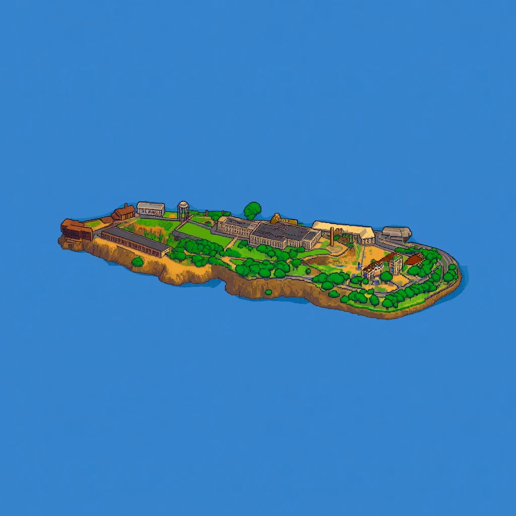
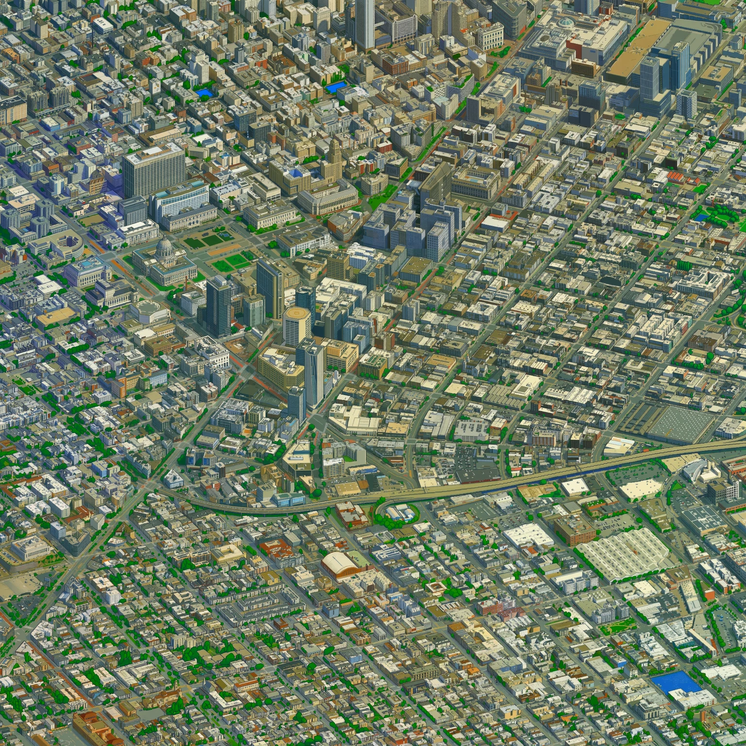
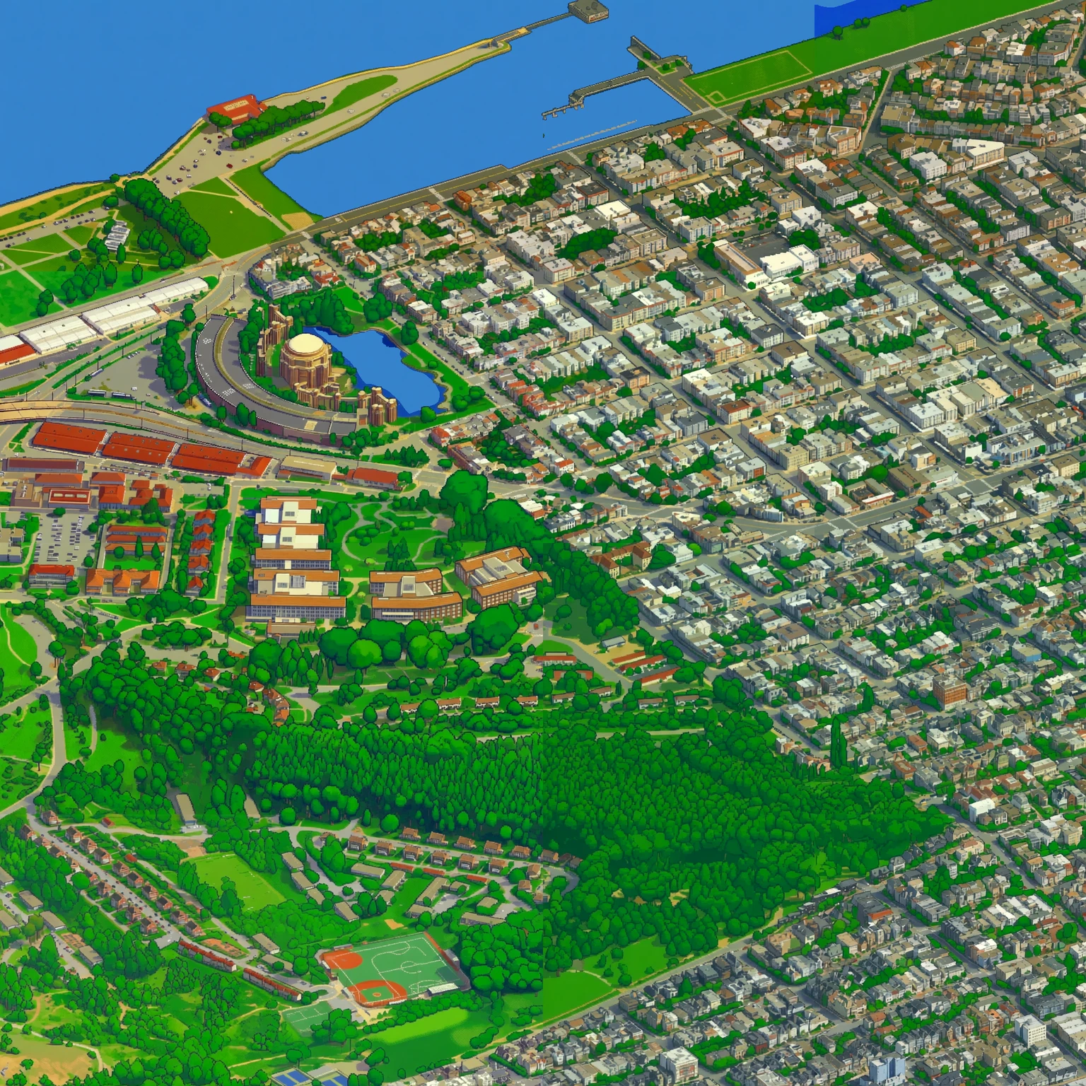
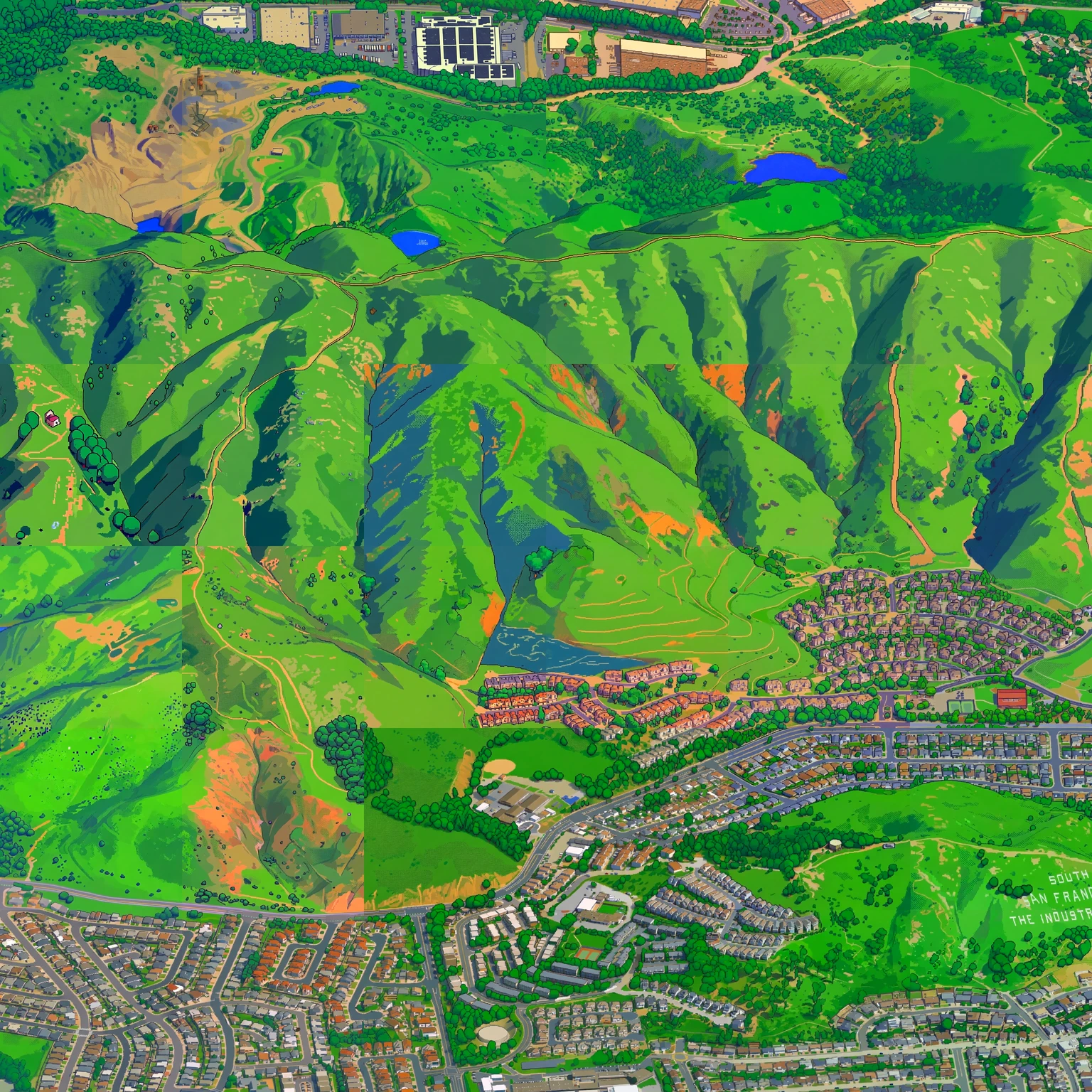
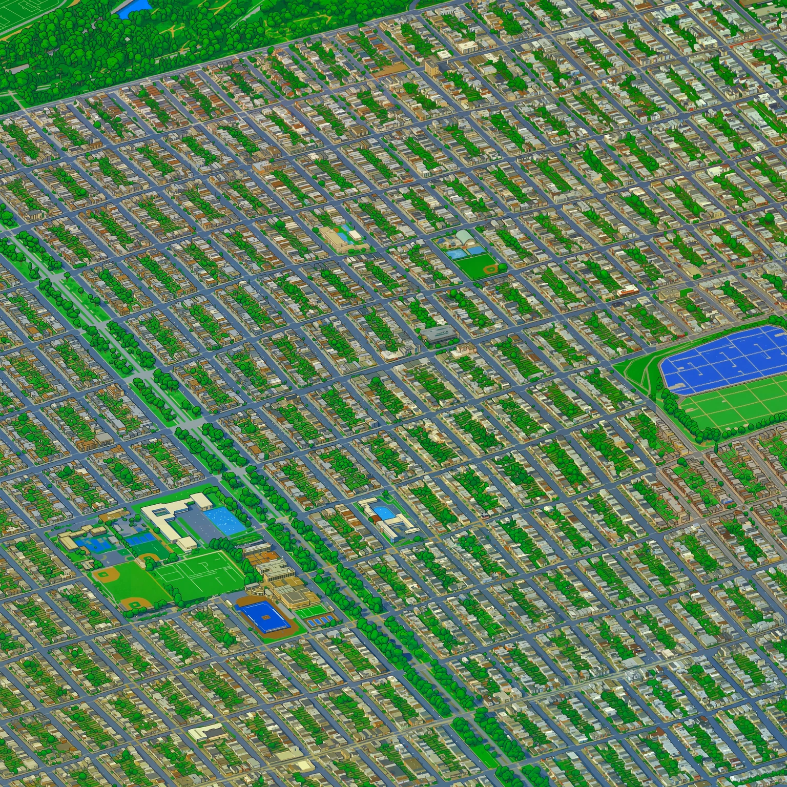
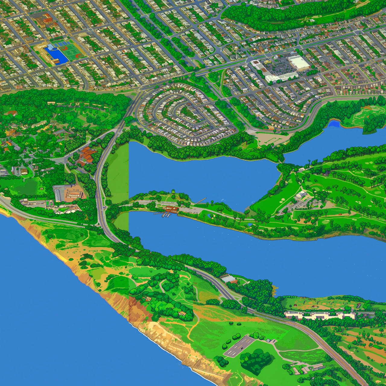
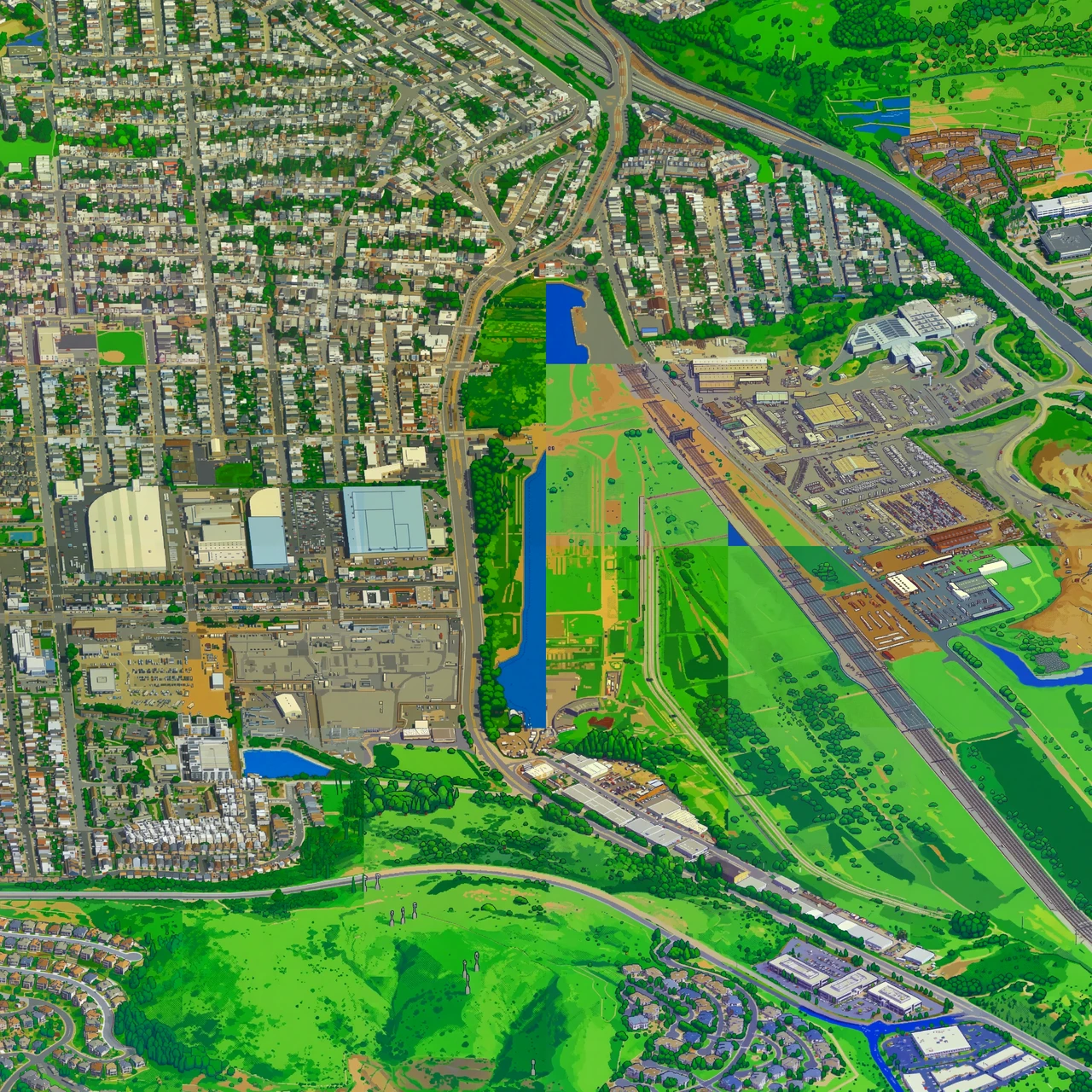
SF imagined by Qwen Image Edit 2511, fine-tuned on 3D Google Map renders. Inspired by isometric.nyc, an homage to Silicon Valley, built with my ragtag team of clankers. Welcome to the golden age of side-projects.
This page is a log of the dev process, roadblocks and lessons learned. About ~90% human-written.

0Why [Why not!?]
Isopolis is by far my most ambitious side-project to date. Throughout this report, you'll see how I would have either not attempted this project, or abandoned it at least 10 times without coding agents. If it feel like I am gushing over them, it is because I am. I'm stoked for the golden era of side-projects!
Isopolis is a continuous, zoomable, clickable isometric pixel-art map of SF. All ~121 km² of it which works out to roughly a 22-gigapixel image. A few months ago, I saw isometric.nyc and was immediately sold on making it for SF. Also, I wanted to recreate the opening credits scene of Silicon Valley show, which was as hilarious as it was accurate. I started with a simple plan to just replicate the NY pipeline, for SF. Poor, naive me.
The basic idea is simple: we can train a tiny LORA on a few ground truth pairs of 3D map render and ghiblified image, then run the model over the whole city. Each part of the pipeline, was supposed to be easy.
Steps:
- Get the 3D google tiles of SF
- Generate a few ground truth pairs of 3D render and ghiblified image via some SOTA image model
- Train a LORA on those pairs
- Run the model over the whole city (with some inference strategy to ensure continuous style)
- Make maptiles out of the generated images
- Build a snazzy app around it
- ... PROFIT???

1Data
1aRendering the city
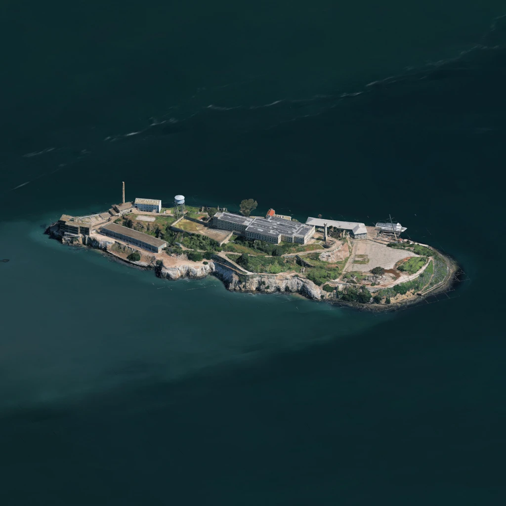
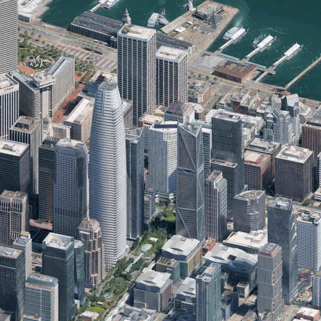
The source is Google Photorealistic 3D Tiles. Isometric.nyc explored and rejected the use of 3d building data. It is pretty insane that US gov has free LIDAR data for every city in the US available to the public. I spent <30mins exploring this and stuck to google 3d images. Claude Code whipped up a scraper to stream the 3D Tiles and render with three.js. This gives the best "real" texture base for the model to learn from. Anything else would involve a LOT of manual work to get the inputs right.
All map math happens in a single fixed local ENU tangent plane. The camera is orthographic, azimuth 22.5°, elevation 30°. I chose it by eye from comparison renders after a few trials. This was all vibes based, no real science here. The intended effect was a classic Sim City view of the city. The Ground point (e, n, h) → map pixel math works out roughly so:
The capture process was basically Playwright driving the three.js page headless, a worker pool rendering blocks in parallel. The tiles' textures have baked lighting. Shading them again would double-light the city. I learnt this the hard way. There are errors that build up with the single camera over the whole city, but they are negligible at our city scale. In the end, we ended up with 440 blocks of 1024² renders.

Roadblocks: Speed, errors.
This sort of scraping is actually against Google's TOS. So the process was painfully slow and error-prone. The workers often got rate-limited. But Claude Code prevailed! I had a loop set up with the error rate and the render time. It was able to go from ~3 mins to ~20 seconds per render.
1bGround truth, with nano banana
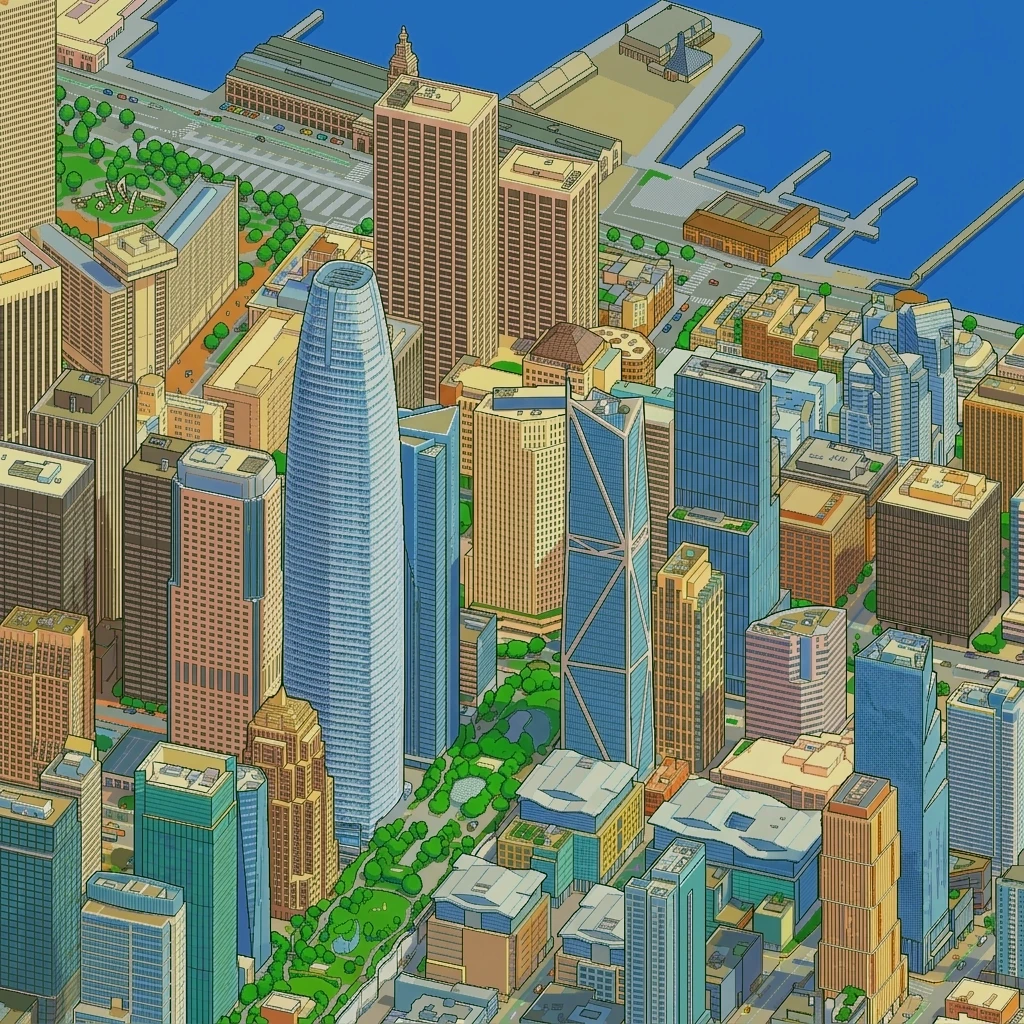
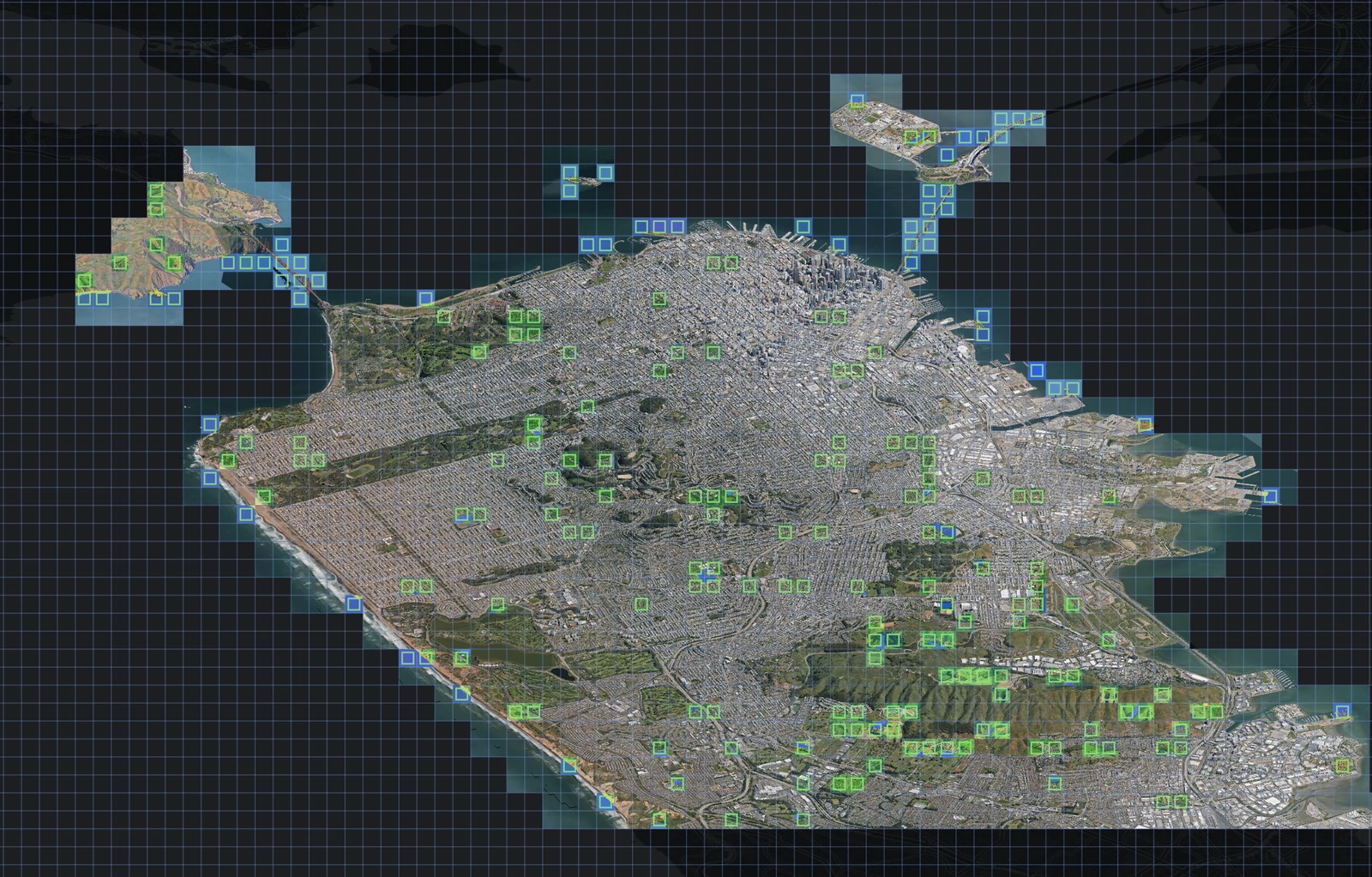
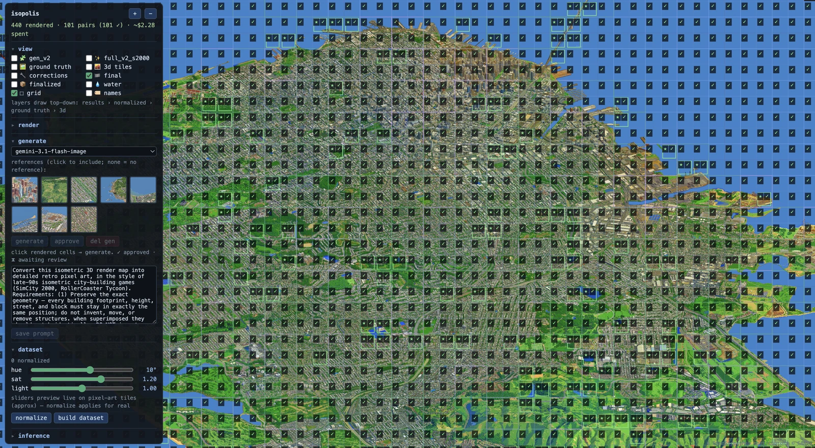
Now that we have the 3D tiles, we need to generate the ground truth pairs for training! Similar to isometric.nyc, I generated a few ghibli-style pixel-art images using Google's Nano Banana. SF terrain is very interesting. There are quite a few distinct features like skyscrapers in FiDi, the hills in the southeast, 2 iconic bridges, lots of coastline, piers, parks, suburban grids and lots of water. I generated a ton of images and curated from them. Getting consistent style was a challenge. There was a LOT of manual trial and error. But as usual, Claude Code added this feature to the dev app that allowed me to select the best images and approve them.
Roadblocks: Style consistency
Getting consistent style was a huge challenge. I spent a ton of time generating 8 reference images using the Pro model. Once I was satisfied with the style, I froze those 8 images and used them as references for all subsequent generations via a smaller model.
I created one training set with ~60 image pairs, and another with ~100. These were the basis for the two training runs we will describe in the next section. The total cost was ~$4 for the image generation.
1cThe training set: masks, normalization, infill
Color normalization. Palette drift across tiles was the NYC project's #1 problem at scale, so I tried to preempt this by color-normalizing the training dataset. I did channel-wise mean-std normalization over the inputs (renders) and outputs (pixel art) separately, then applied the same normalization to every render. Following the NYC precedent, I masked out water and vegetation from the statistics, so the model learns to color-match only the built environment. I also applied a HSV transform to the outputs to give them a a warm, slightly sunny look, and a slight saturation boost.
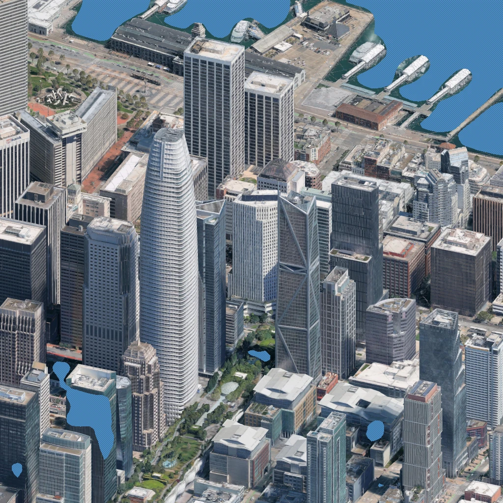
The water problem. Open water in an orthographic render is a hundred thousand near-identical pixels. This texture-less void makes it incredibly difficult for a model to learn water, and it hallucinates structure into it. There was no real solution to this. I tried the checkerboard heuristic from isometric.nyc, but it was too aggressive and rejected shallow water. In the end, I used heuristics to generate a water mask for every image. Then replaced "water" pixels in the input with our "water" color. But even this was not enough, and we had to "adjust the water" in post-processing. The model was still hallucinating structures in the water, and we had to manually remove them.

Roadblocks: Teal water isn't blue water
I calibrated the water gate on deep bay water (hue 190–197, saturation 0.57–0.69), with a saturation floor to reject blue-gray street shadows. Then a Treasure Island tile that is 62% open water sailed through with no mask at all: shallow teal water sits at sat 0.34–0.38, squarely inside the shadow-rejection zone. The saving discriminator is value — teal water is slightly brighter than shadow. The detector now ORs a tight teal branch with the blue branch; six bay tiles gained masks, zero inland tiles changed.

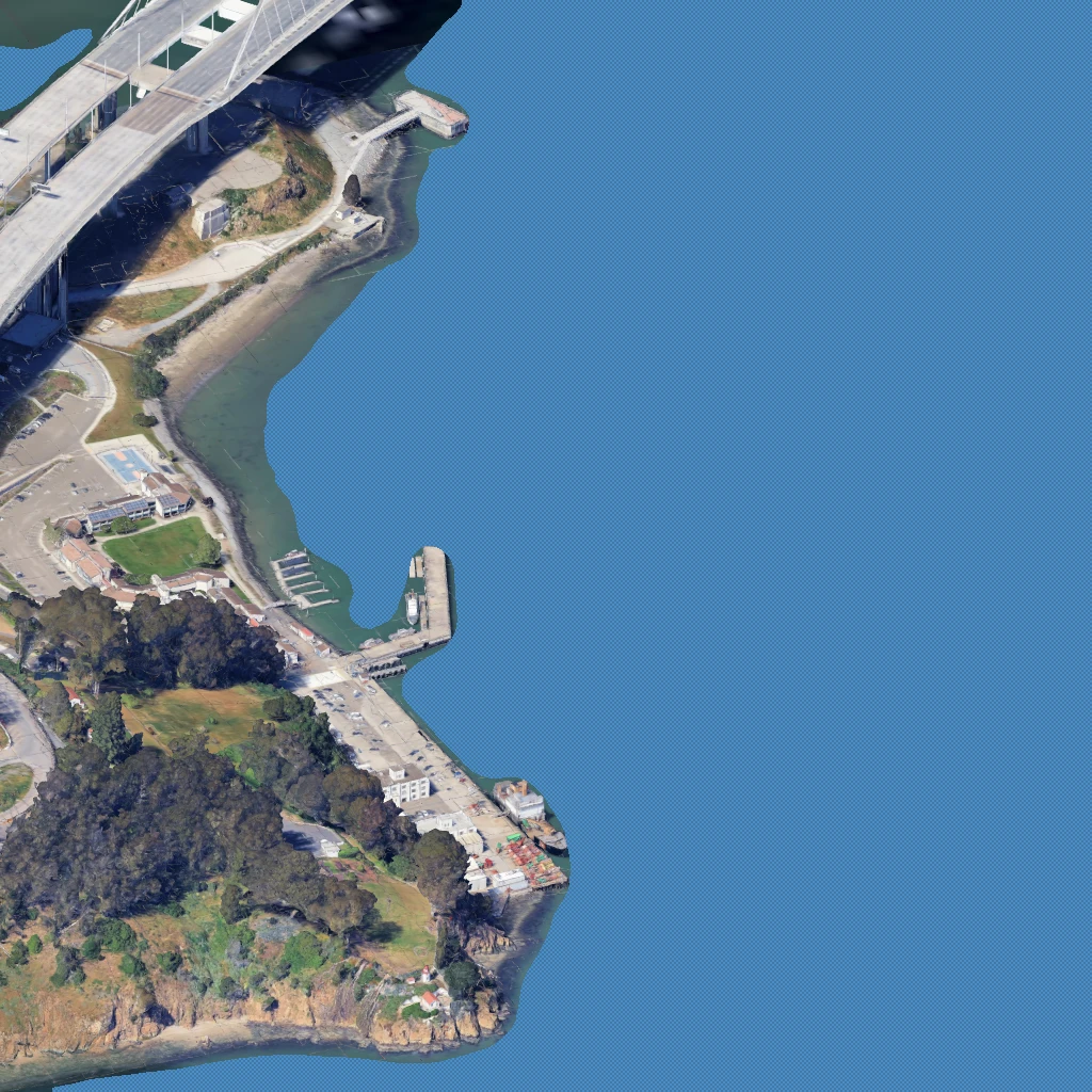
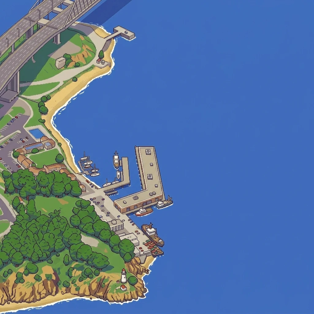
The infill expansion is an extremely important dataset decision, imported wholesale from the NYC post-mortem: the model must learn, from day one, to generate pixel art that continues smoothly. If we just infer all images independantly, there is no guarantee of continuity. What we want is for the model to learn to "extend" the existing pixel art to new, unseen regions. So here's the final training objective. We divide each training example into 4 quadrants, and generate 15 different input patterns for each example. Each pattern is a 4-bit number, where each bit indicates whether the corresponding quadrant is already generated (1) or not (0). The model is trained to generate the missing quadrants based on the existing ones. This way, the model learns to infill missing regions while maintaining continuity with the existing pixel art.
101 pairs × 15 patterns = 1,515 training samples, a few full pairs held out for validation. The expansion doubles as honest augmentation: the model sees each scene under 15 different context regimes.

2Training & inference
2aA LoRA TL;DR
The base model I chose is Qwen-Image-Edit-2511 (Apache 2.0): a 20B-parameter image-to-image model. This is the best open weights model in this weight class, and is trained for exactly the type of task we want: image-to-image translation. I won't go into the details of how LORA works, but the basic idea is that we don't want to fine-tune the whole model on our small dataset. Instead, we want to learn a small set of parameters that can adapt the base model to our specific task.
The base stays entirely frozen. Every attention projection W in its transformer gets a parallel low-rank residual — a LoRA:
with B zero-initialized, so step 0 is exactly the base model. That's ~55M trainable parameters — 0.28% of the transformer — trained with a ~500-line HF trainer I rolled by hand (diffusers + peft + accelerate, no trainer framework). The frozen conditioning encoders (a 7B vision-language model + a VAE) run once in a prep pass and get cached, so training-step time is pure transformer.
The LORA is ~200 MB as opposed to the base model's 40 GB weights.
2bModal
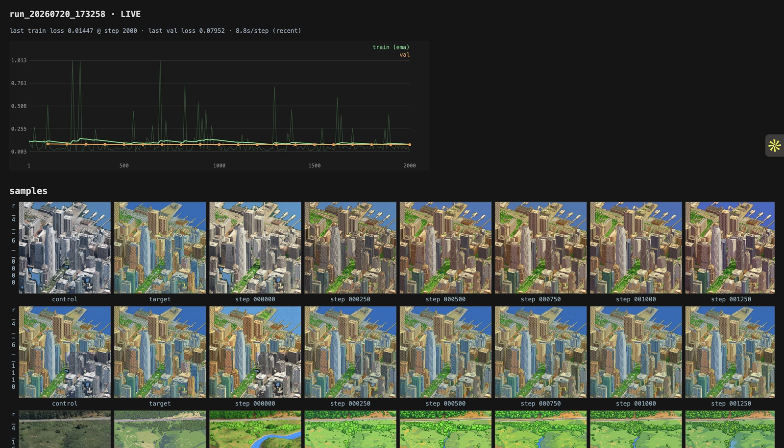
Everything GPU-shaped runs on Modal's serverless H100s. I had never used Modal before, but it was nothing Codex couldn't handle. First I uploaded all images to a Modal volume, then ran the prep pass to cache the frozen encoders. I then ran two training runs, one on the 60-pair dataset and one on the 100-pair dataset. Each run took ~2–3 hours and cost ~$10–15. The training was done with a batch size of 1 and gradient accumulation of 4, using bf16 precision. The evaluation cadence was set to compute validation loss every 100 steps and generate a preview grid every 250 steps. The sampling during inference used true CFG with a scale of 4.0 and 24 Euler steps, which is exactly what inference uses.
| hardware | 1× H100-80GB · ~$4/hour |
| a full training run | 2,000 steps · bs 1 × grad-accum 4 · bf16 · ≈ 2–3 h ≈ $10–15 |
| eval cadence | val loss every 100 steps (frozen noise draws) · preview grid every 250 |
| sampling | true CFG, scale 4.0 · 24 Euler steps — exactly what inference uses |
Loss is just a proxy and the curve mostly measures how hard the conditioning is working. The most important signal is the preview grid: fixed inputs (favorites + held-out pairs, from-scratch and infill patterns) sampled at step 0 as a base-model baseline, then every 250 steps. A deployed monitor serves this live report during a run.
2cInference
Once I had the trained models, I ran inference on the entire city. These are not the final images, but it was a good sanity check to see if the model was producing reasonable outputs. There was no "strategy" here, I just gave the model the 3D render and let it generate the pixel art. The results were promising, but as expected, there were a ton of issues:
- No continuity between adjacent blocks
- Color palette drift across blocks
- Hallucinations in water and vegetation
- Style inconsistencies
Also, the 100-pair model was better than the 60-pair model, so that was a straightforward choice. We had to figure out how to solve the continuity and style issues.
2dThe overlap plan
Independently generated blocks already sort of agree geometrically as every render shares one global frame. A freeway drawn in one block continues into the next at the right pixels. What they don't share is style state, and palette. The fix was to generate images via a sliding window. We first run inference on an image. Then, we slide by half image in any direction, and generate the next image. This closely matches the training objective! Remember the compositing 15 training patterns?
I generated a handful "seed" generations from our inference run. Claude Code then wrote a seam planner that greedily grows the rest of the city from those seeds, always generating a new window with at least one quadrant already generated. The model sees the existing pixel art as context, and the new window is generated to match it. This way, we can ensure continuity across the entire city (at least in theory).
There are two disadvantages still:
- The generation is extremely slow since each generation is effectively a DAG.
- There are still some continuity issues, especially where 2 adjacent windows collide.
- 440 generations now become 1,519 generations in 67 waves (due to overlapping windows).
One guard Codex suggested was to compare each generation against our baseline inference run. If the new generation is too different from the baseline, we can reject it and try again.
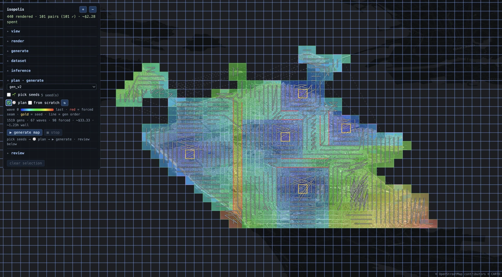

Roadblocks: a city upon the water
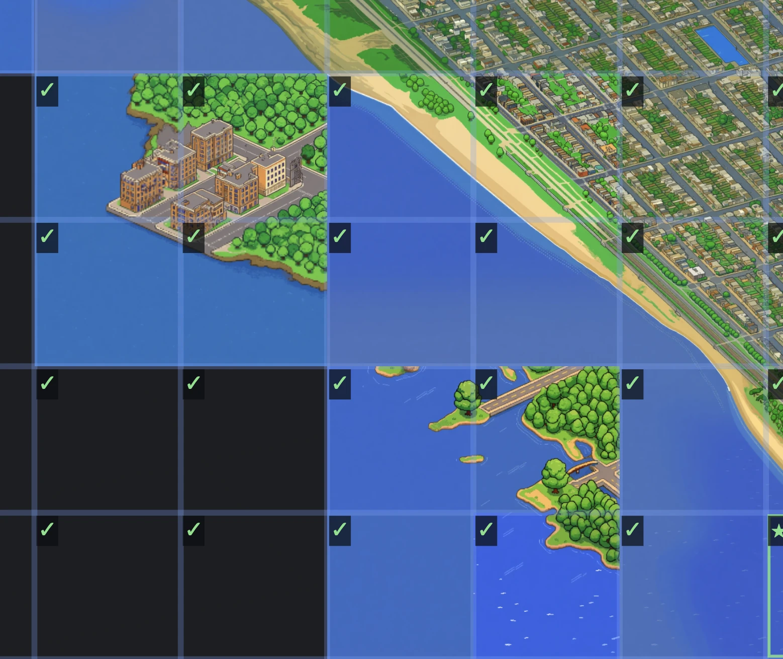
As predicted, any window that was mostly ocean was out of distribution. When asked to fill the void, the model confidently generated more city. My fix was three-sided: I skipped windows above a water threshold entirely (they now get stamped, §3b).

3Maptiling
3aManual checking
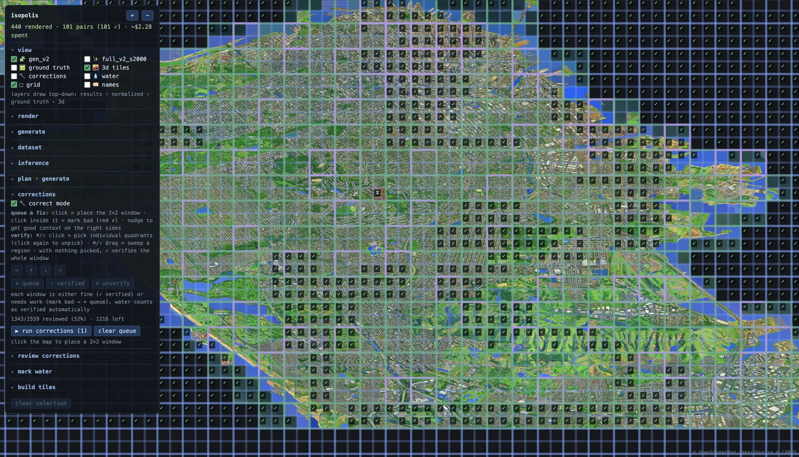
I reviewed the generated map the same way I curated the dataset: me, a map, and a flag button. Codex added all quadrants to the map. The v2 sweep finished 1,606 generated quadrants with 8.3% falling back to defensive behavior. Review was genuinely pretty fast (~1hr). I flagged ~200 quadrants for correction.
3bRegenerations
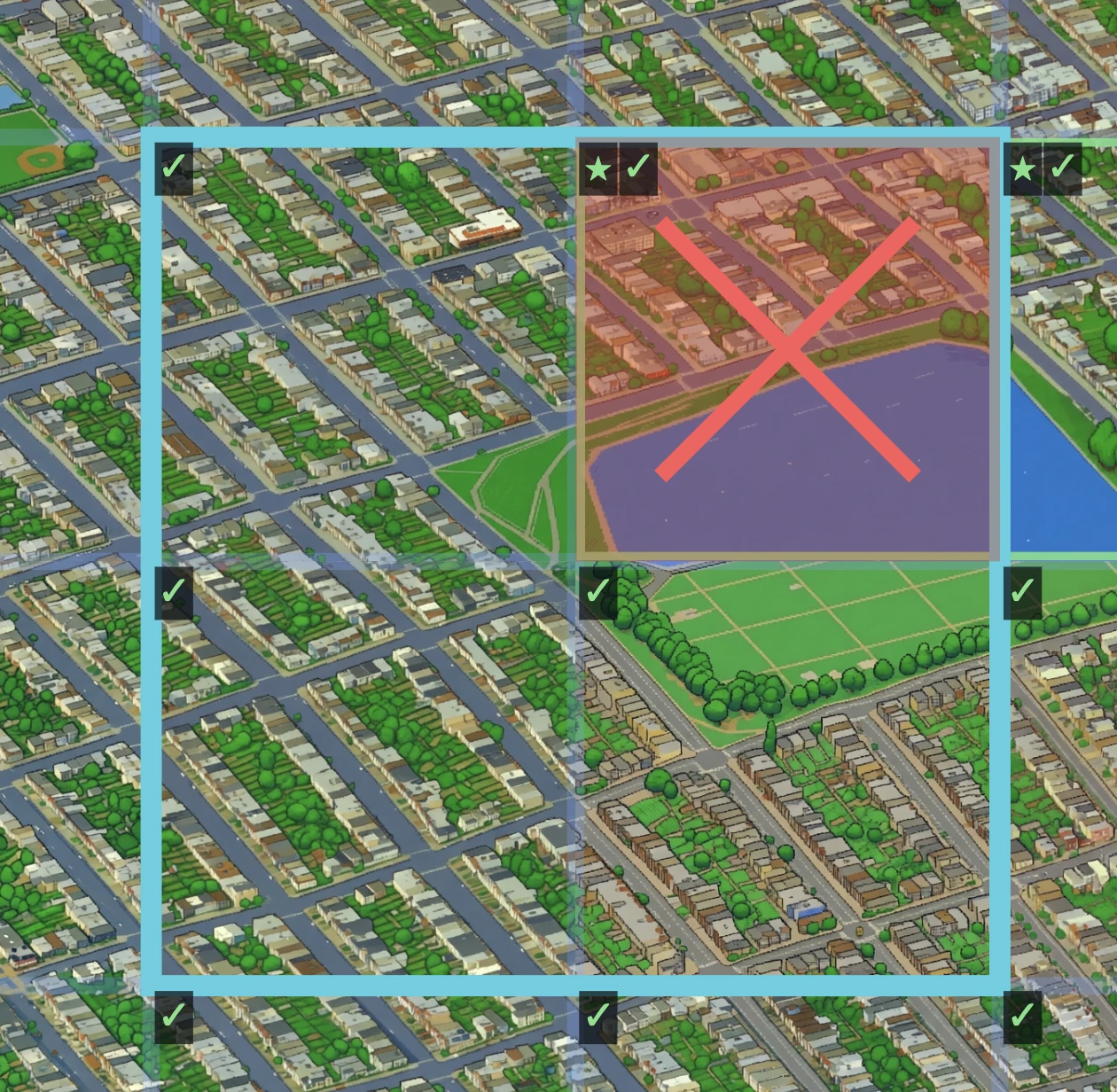
One great thing about having random errors is that I could now use arbitrary context to fix them. As long as the surrounding quadrants were good, I could regenerate a bad quadrant with the good ones as context.
Fable here built the pipeline to create this new input dataset, perform the inference, and then cut out the new quadrants and put them back into the map. I then reviewed the new quadrants and repeated this process until all quadrants were verified.

what went wrong · the bridge goes to nano banana
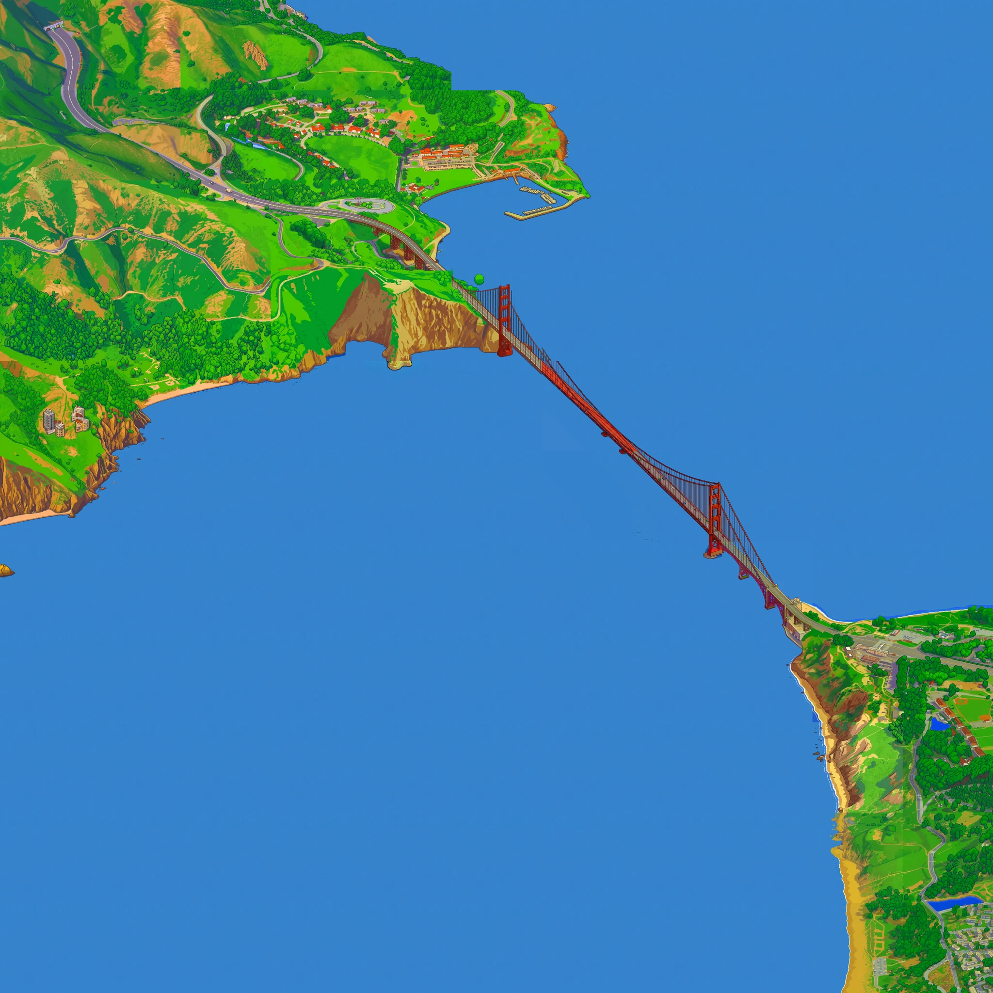
The golden gate bridge is a very distinctive landmark, and was extremely out of distribution for the model. I had to finally give up and use Nano banana to generate 50% of the bridge unconnected to the rest of the city. The model was hallucinating a lot of extra structure and the bridge was not recognizable.
3cThe water stamp
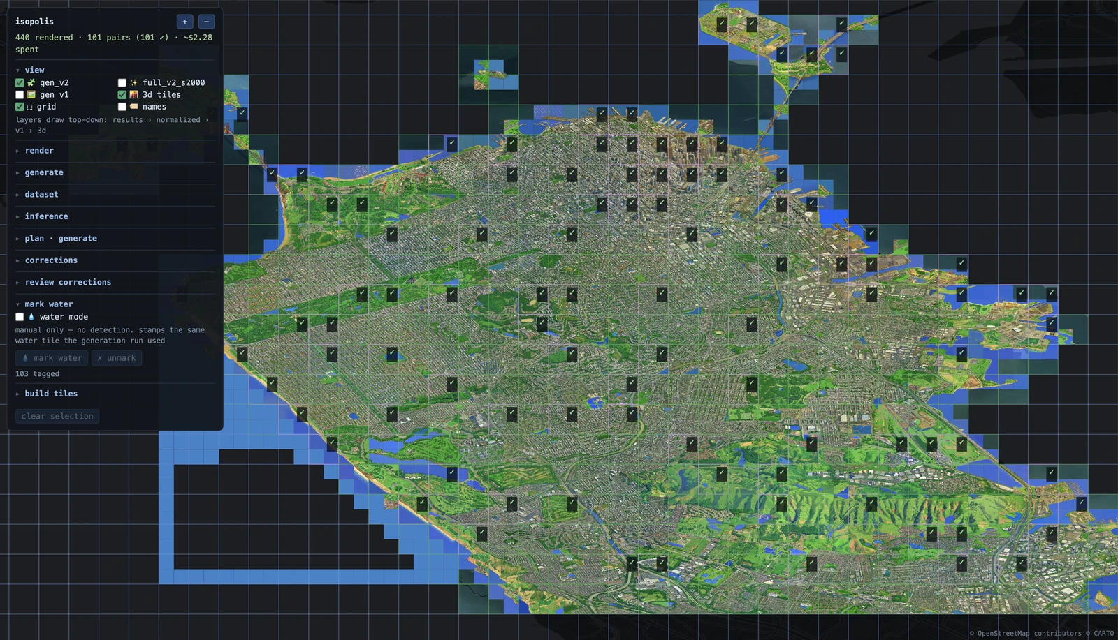
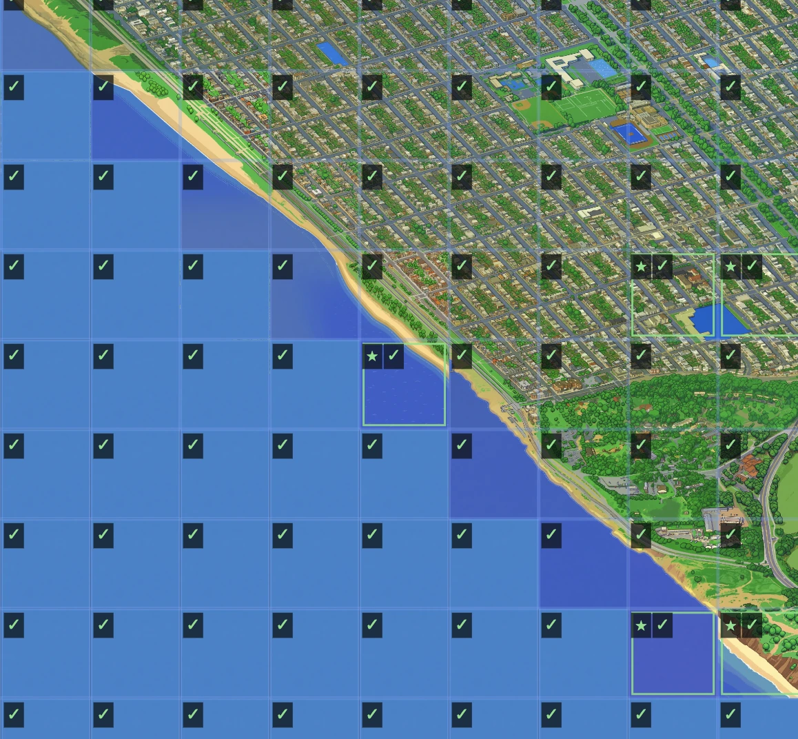
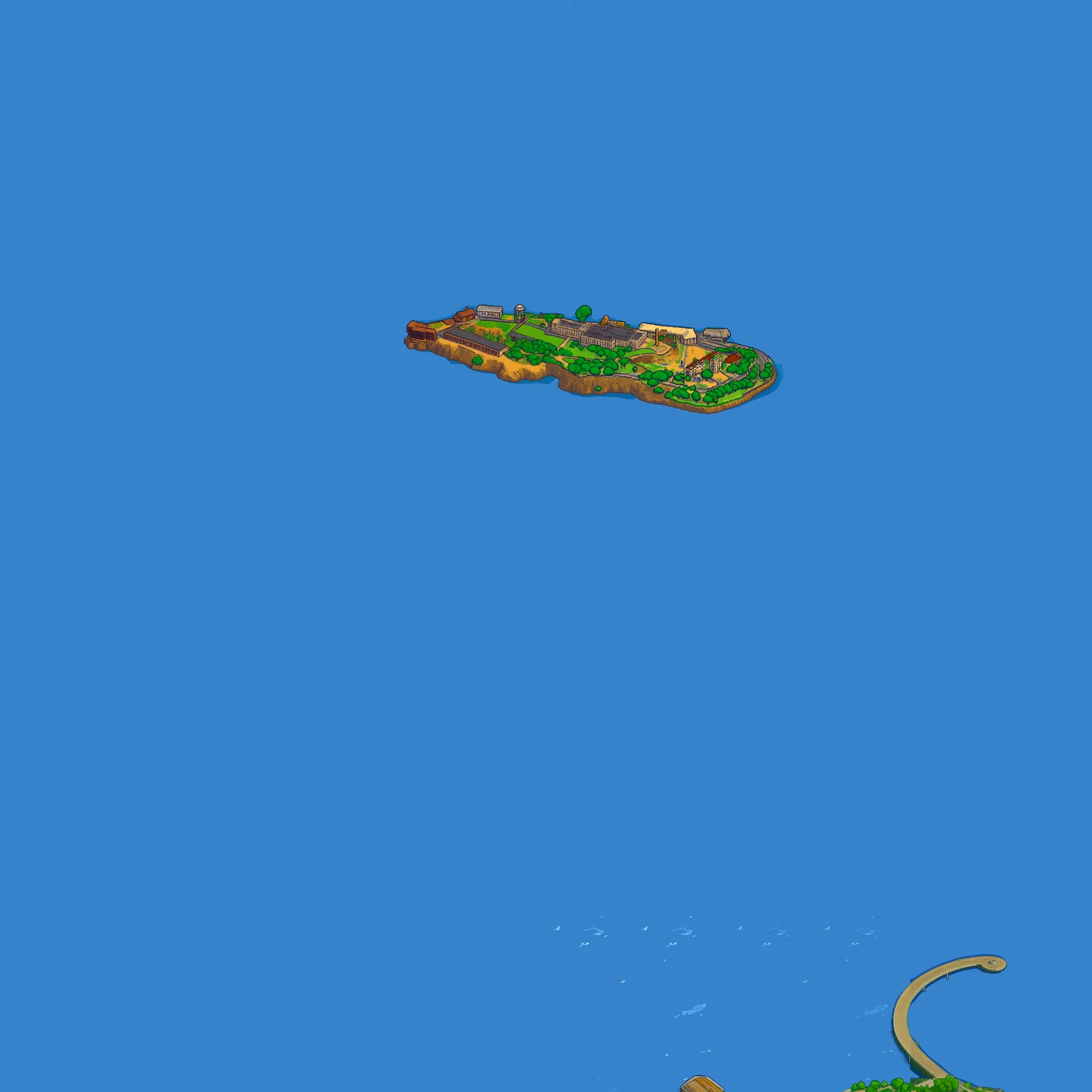
The bay area has large swaths of open water. For this, we added a feature to the ops app to stamp water tiles. We selected large regions and filled them with a single water tile. These were 100% water tiles.
For tiles that had some water and some land, we used the water mask to determine which pixels should be water. We used heuristics to determine the mask, and then stamped the water tile on top of the generated pixel art via the mask. This way, we could ensure that all water tiles were consistent and matched the rest of the city.
3dThe tile pyramid
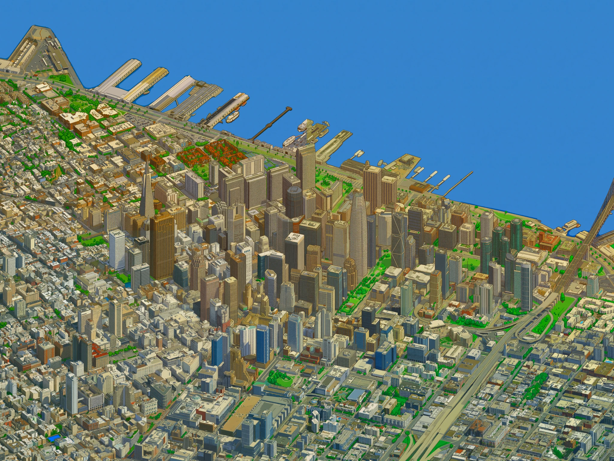
The published set comprises of2,630 quadrants: 1,606 generated, 1,024 water stamps. I generated a classic map-serving tile pyramid. Level-0 tiles are the quadrants themselves; each level up BOX-downsamples 2×2 children into one parent, nine levels in all.

4The viewer
4aThe app
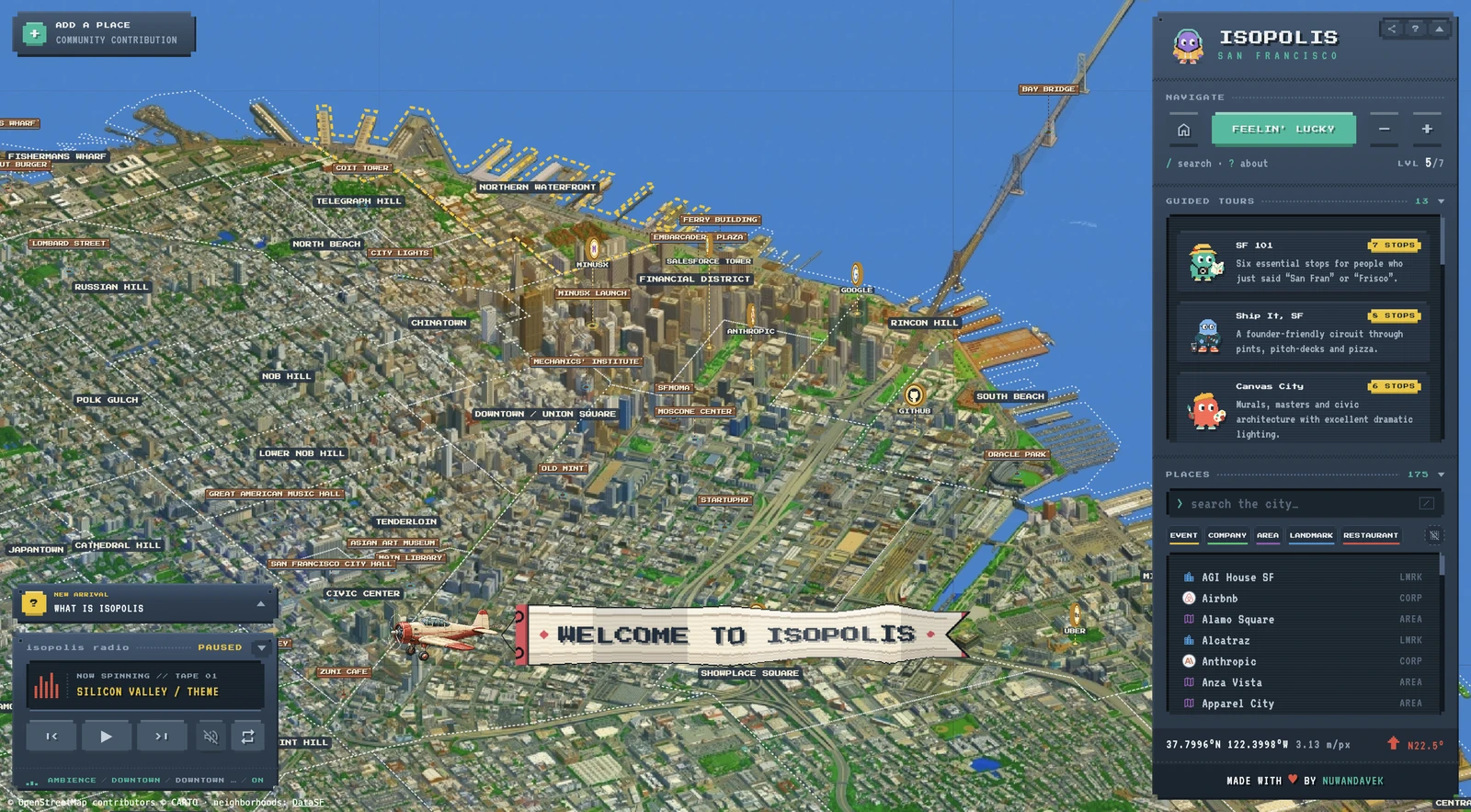
I (Codex, mostly)wrote the viewer without a map library. This map is a fixed local-ENU dimetric projection, not Mercator. MapLibre or deck.gl would resample the pixel art through a projection it was never drawn in and still couldn't index tiles into this view. So the core is a small canvas engine I rolled by hand. Underneath everything, CARTO's dark basemap tiles are warped into the dimetric frame at 45% alpha, which is what lets you zoom out from pixel-art San Francisco to a whole recognizable Bay Area. Over that is the pixel art tile pyramid, which is drawn in a single pass.
Everything on top is data, not code: annotations are GeoJSON ([lon, lat, h], projected to map pixels at load) — signposts, company coins, sprites, neighborhood polygons, tours. The whole app state lives in the URL hash (#@lat,lon,scalez/…), so every view, selection and tour stop is a shareable link. I am particularly excited about the tours. Codex whipped up nice little mascots for each tour, and used OSM data to generate a path through the city. Silicon valley opening credits music plays as you open the app! I am particularly proud of the ambient soundscape, I will let you discover it for yourself.
The whole thing is static files. S3 + CloudFront is the hosting.
5What's next
- Figure out a way to fix remaining seam bugs. A few harsh boundaries and inconsistent continuations survived in random places. This should be fixed. Better model? better dataset? better seam planner? better seam blending? Not sure, but I have some ideas.
- More styles. The whole point of the LoRA architecture is that a winter map or a night map is one more ~200 MB adapter over the same frozen base, not a new pipeline.
- More cities? The pipeline is geo agnostic and easily extensible to other cities.
- Better tours. I want to add more tours, and also add a way to checkout events? IT would be cool if this becomes a living map of the Bay Area, with events and tours and maybe even a way to add your own content.
7Reading & credits
Reading
- isometric.nyc: the inspiration, and the post-mortem this project is built on.
- Hu et al., LoRA: low-rank adaptation
- Liu et al., Rectified Flow and Lipman et al., Flow Matching: the training objective.
- Esser et al., SD3: the MMDiT transformer family the base model belongs to.
- Qwen-Image technical report: the base model itself.
Credits
- 3D city data: Google Photorealistic 3D Tiles, rendered with 3d-tiles-renderer + three.js.
- Context basemap: CARTO · © OpenStreetMap contributors.
- Neighborhood boundaries: SF Find Neighborhoods (public domain).
- YC startup data & logos: YC Startup Map.
- Company logos: Simple Icons. UFOs: CC0, opengameart.org.
- Type: Press Start 2P & VT323, Google Fonts.
- Coding agents: Claude Opus 5 (~30% of code), Claude Fable 5 (~40% of code) and GPT-5.6-Sol (~30% of code) wrote most of this code. In a real sense the project would have been impossible without them. Me doing it alone would have taken 10x as long, and it would almost certainly still sit unfinished somewhere around step two. Code quality wasn't great, but these agents figured things out that would have taken me much much longer on my own. A significant portion of my work was in the meta programming, and imbibing taste throughout the project squinting over the map with a fine tooth comb.